
Within the first put up on this collection, we launched the usage of hashing methods to detect related capabilities in reverse engineering situations. We described PIC hashing, the hashing approach we use in SEI Pharos, in addition to some terminology and metrics to judge how properly a hashing approach is working. We left off final time after exhibiting that PIC hashing performs poorly in some instances, and puzzled aloud whether it is potential to do higher.
On this put up, we are going to attempt to reply that query by introducing and experimenting with a really totally different kind of hashing known as fuzzy hashing. Like common hashing, there’s a hash perform that reads a sequence of bytes and produces a hash. In contrast to common hashing, although, you do not examine fuzzy hashes with equality. As a substitute, there’s a similarity perform that takes two fuzzy hashes as enter and returns a quantity between 0 and 1, the place 0 means fully dissimilar and 1 means fully related.
My colleague, Cory Cohen, and I debated whether or not there’s utility in making use of fuzzy hashes to instruction bytes, and our debate motivated this weblog put up. I assumed there can be a profit, however Cory felt there wouldn’t. Therefore, these experiments. For this weblog put up, I will be utilizing the Lempel-Ziv Jaccard Distance fuzzy hash (LZJD) as a result of it is quick, whereas most fuzzy hash algorithms are sluggish. A quick fuzzy hashing algorithm opens up the potential of utilizing fuzzy hashes to seek for related capabilities in a big database and different attention-grabbing prospects.
As a baseline I am going to even be utilizing Levenshtein distance, which is a measure of what number of modifications you should make to at least one string to rework it to a different. For instance, the Levenshtein distance between “cat” and “bat” is 1, since you solely want to vary the primary letter. Levenshtein distance permits us to outline an optimum notion of similarity on the instruction byte stage. The tradeoff is that it is actually sluggish, so it is solely actually helpful as a baseline in our experiments.
Experiments in Accuracy of PIC Hashing and Fuzzy Hashing
To check the accuracy of PIC hashing and fuzzy hashing below varied situations, I outlined a number of experiments. Every experiment takes the same (or similar) piece of supply code and compiles it, generally with totally different compilers or flags.
Experiment 1: openssl model 1.1.1w
On this experiment, I compiled openssl model 1.1.1w in a number of other ways. In every case, I examined the ensuing openssl executable.
Experiment 1a: openssl1.1.1w Compiled With Totally different Compilers
On this first experiment, I compiled openssl 1.1.1w with gcc -O3 -g and clang -O3 -g and in contrast the outcomes. We’ll begin with the confusion matrix for PIC hashing:
|
|
|
|
|
|
|
|
|
|
|
|
As we noticed earlier, this ends in a recall of 0.07, a precision of 0.45, and a F1 rating of 0.12. To summarize: fairly unhealthy.
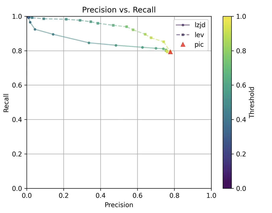
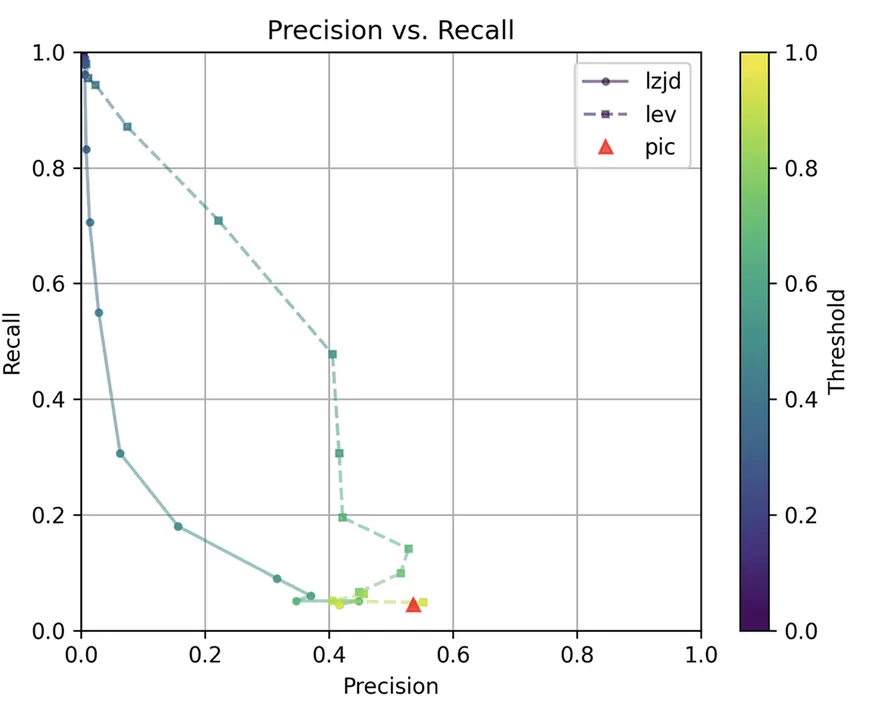
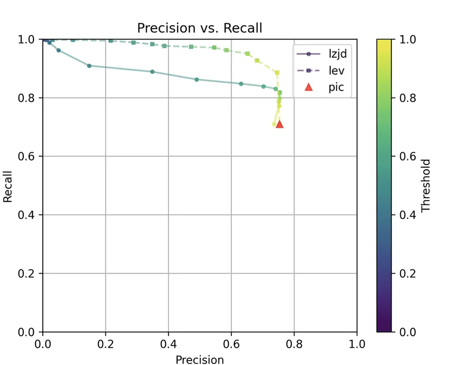
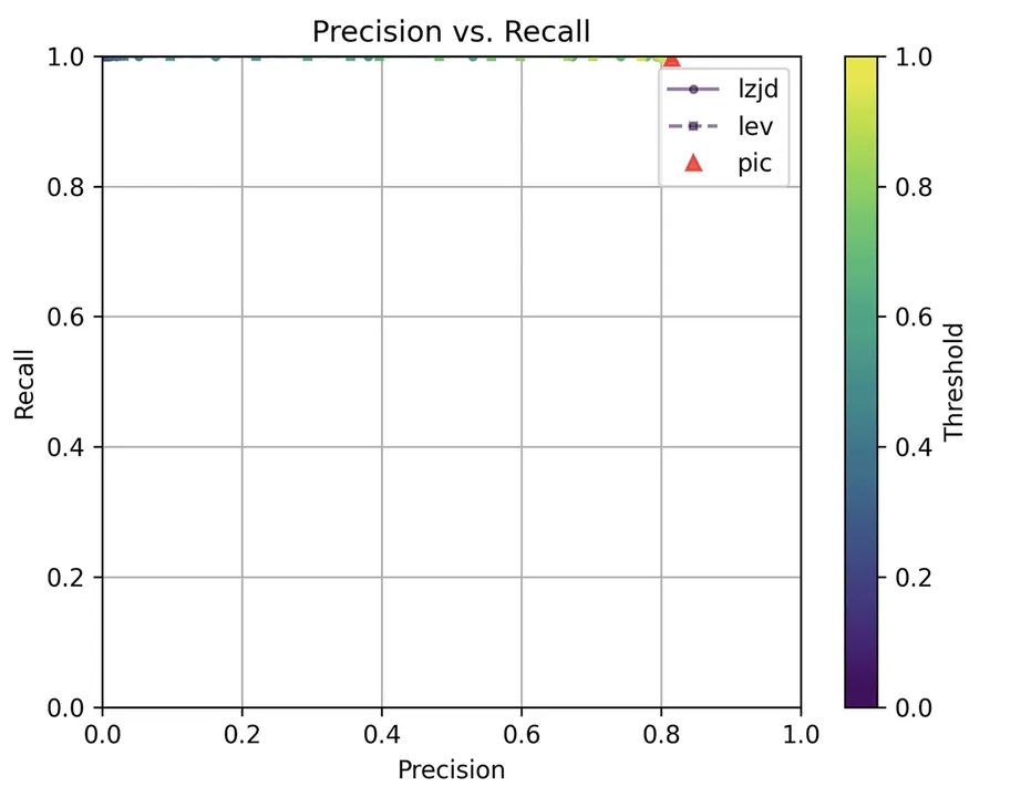
How do LZJD and Levenshtein distance do? Nicely, that is a bit tougher to quantify, as a result of we’ve got to select a similarity threshold at which we contemplate the perform to be “the identical.” For instance, at a threshold of 0.8, we might contemplate a pair of capabilities to be the identical if that they had a similarity rating of 0.8 or larger. To speak this info, we might output a confusion matrix for every potential threshold. As a substitute of doing this, I am going to plot the outcomes for a spread of thresholds proven in Determine 1 beneath:
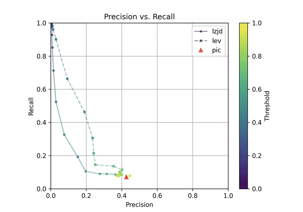
Determine 1: Precision Versus Recall Plot for “openssl GCC vs. Clang”
The pink triangle represents the precision and recall of PIC hashing: 0.45 and 0.07 respectively, identical to we calculated above. The strong line represents the efficiency of LZJD, and the dashed line represents the efficiency of Levenshtein distance (LEV). The colour tells us what threshold is getting used for LZJD and LEV. On this graph, the perfect consequence can be on the prime proper (one hundred pc recall and precision). So, for LZJD and LEV to have a bonus, it ought to be above or to the proper of PIC hashing. However, we are able to see that each LZJD and LEV go sharply to the left earlier than shifting up, which signifies {that a} substantial lower in precision is required to enhance recall.
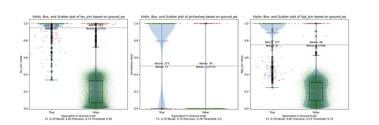
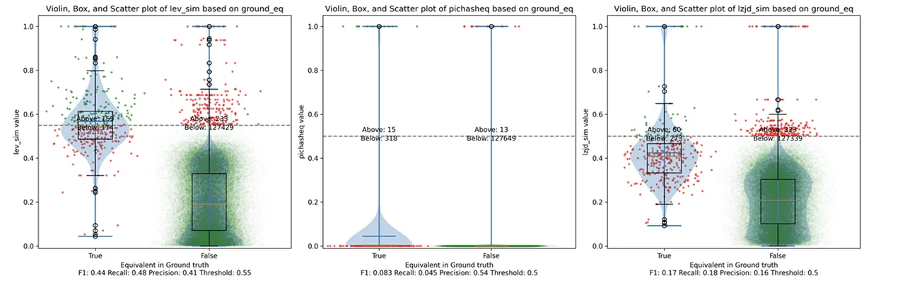
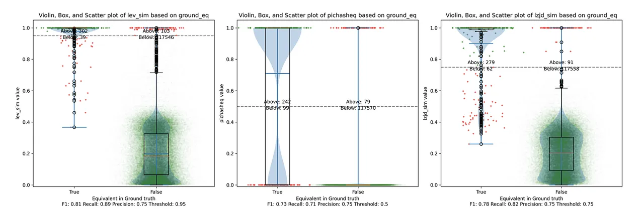
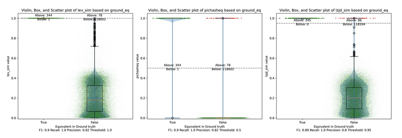
Determine 2 illustrates what I name the violin plot. Chances are you’ll wish to click on on it to zoom in. There are three panels: The leftmost is for LEV, the center is for PIC hashing, and the rightmost is for LZJD. On every panel, there’s a True column, which reveals the distribution of similarity scores for equal pairs of capabilities. There may be additionally a False column, which reveals the distribution scores for nonequivalent pairs of capabilities. Since PIC hashing doesn’t present a similarity rating, we contemplate each pair to be both equal (1.0) or not (0.0). A horizontal dashed line is plotted to indicate the edge that has the very best F1 rating (i.e., mixture of each precision and recall). Inexperienced factors point out perform pairs which are appropriately predicted as equal or not, whereas pink factors point out errors.
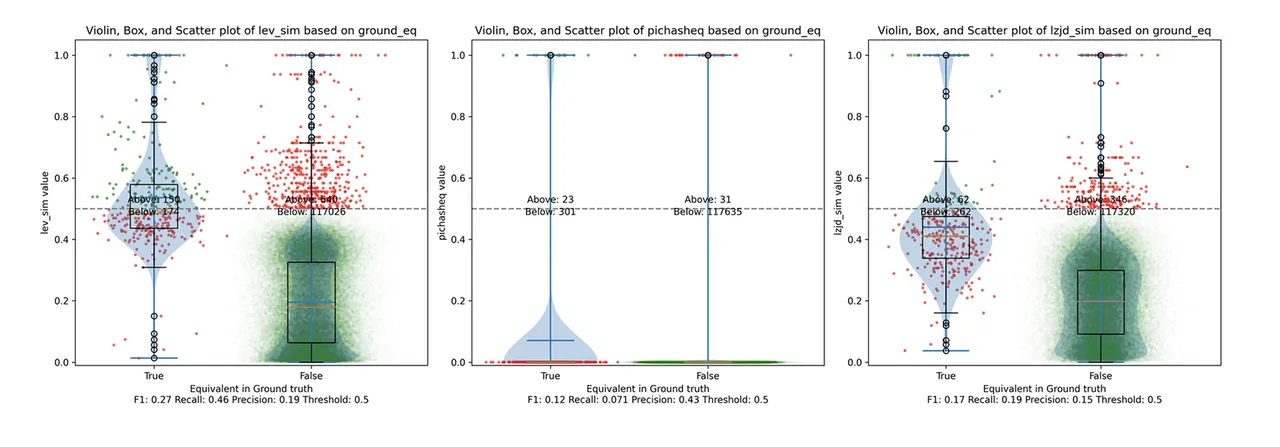
Determine 2: Violin Plot for “openssl gcc vs clang”. Click on to zoom in.
This visualization reveals how properly every similarity metric differentiates the similarity distributions of equal and nonequivalent perform pairs. Clearly, the hallmark of similarity metric is that the distribution of equal capabilities ought to be larger than nonequivalent capabilities. Ideally, the similarity metric ought to produce distributions that don’t overlap in any respect, so we might draw a line between them. In apply, the distributions often intersect, and so as a substitute we’re pressured to make a tradeoff between precision and recall, as may be seen in Determine 1.
General, we are able to see from the violin plot that LEV and LZJD have a barely larger F1 rating (reported on the backside of the violin plot), however none of those methods are doing an awesome job. This means that gcc and clang produce code that’s fairly totally different syntactically.
Experiment 1b: openssl 1.1.1w Compiled With Totally different Optimization Ranges
The subsequent comparability I did was to compile openssl 1.1.1w with gcc -g and optimization ranges -O0, -O1, -O2, -O3.
Evaluating Optimization Ranges -O0 and -O3
Let’s begin with one of many extremes, evaluating -O0 and -O3:
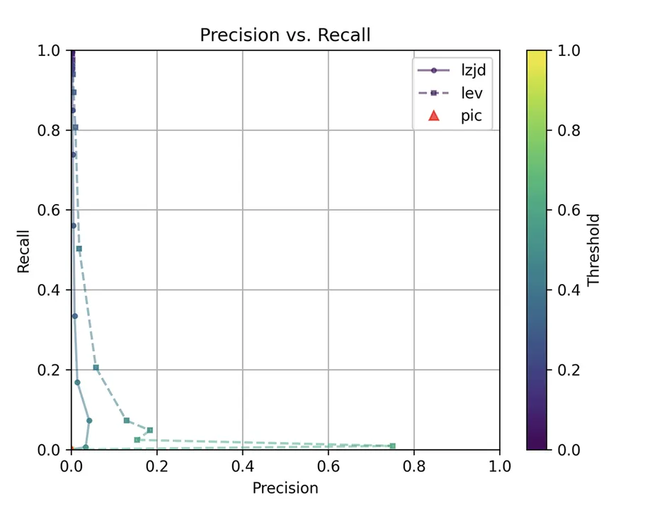
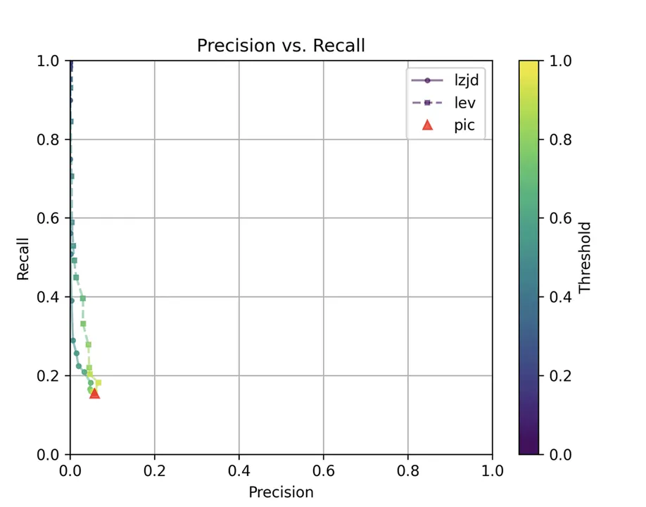
Determine 3: Precision vs. Recall Plot for “openssl -O0 vs -O3”
The very first thing you could be questioning about on this graph is, The place is PIC hashing? Nicely, should you look intently, it is there at (0, 0). The violin plot offers us somewhat extra details about what’s going on.
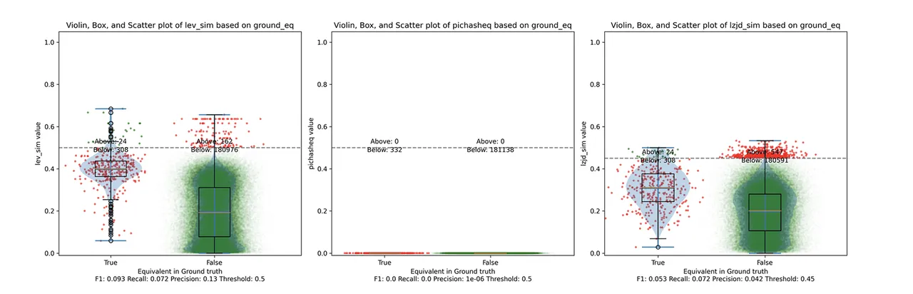
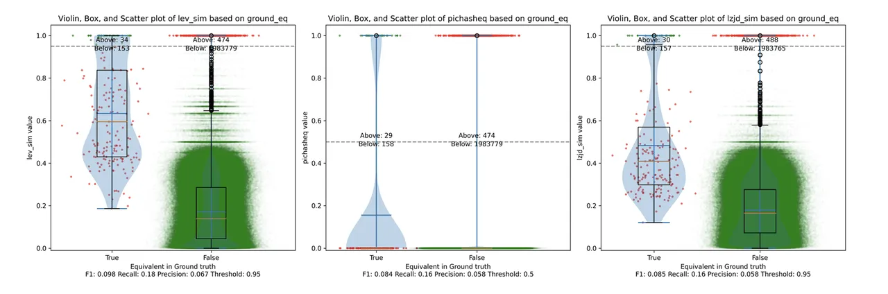
Determine 4: Violin Plot for “openssl -O0 vs -O3”. Click on to zoom in.
Right here we are able to see that PIC hashing made no optimistic predictions. In different phrases, not one of the PIC hashes from the -O0 binary matched any of the PIC hashes from the -O3 binary. I included this experiment as a result of I assumed it could be very difficult for PIC hashing, and I used to be proper. However, after some dialogue with Cory, we realized one thing fishy was happening. To realize a precision of 0.0, PIC hashing cannot discover any capabilities equal. That features trivially easy capabilities. In case your perform is only a ret there’s not a lot optimization to do.
Finally, I guessed that the -O0 binary didn’t use the -fomit-frame-pointer possibility, whereas all different optimization ranges do. This issues as a result of this feature modifications the prologue and epilogue of each perform, which is why PIC hashing does so poorly right here.
LEV and LZJD do barely higher once more, attaining low (however nonzero) F1 scores. However to be honest, not one of the methods do very properly right here. It is a troublesome downside.
Evaluating Optimization Ranges -O2 and -O3
On the a lot simpler excessive, let’s take a look at -O2 and -O3.
Determine 5: Precision vs. Recall Plot for “openssl -O2 vs -O3”
Determine 6: Violin Plot for “openssl -O1 vs -O2”. Click on to zoom in.
PIC hashing does fairly properly right here, attaining a recall of 0.79 and a precision of 0.78. LEV and LZJD do about the identical. Nonetheless, the precision vs. recall graph (Determine 11) for LEV reveals a way more interesting tradeoff line. LZJD’s tradeoff line shouldn’t be practically as interesting, because it’s extra horizontal.
You can begin to see extra of a distinction between the distributions within the violin plots right here within the LEV and LZJD panels. I am going to name this one a three-way “tie.”
Evaluating Optimization Ranges -O1 and -O2
I might additionally count on -O1 and -O2 to be pretty related, however not as related as -O2 and -O3. Let’s examine:
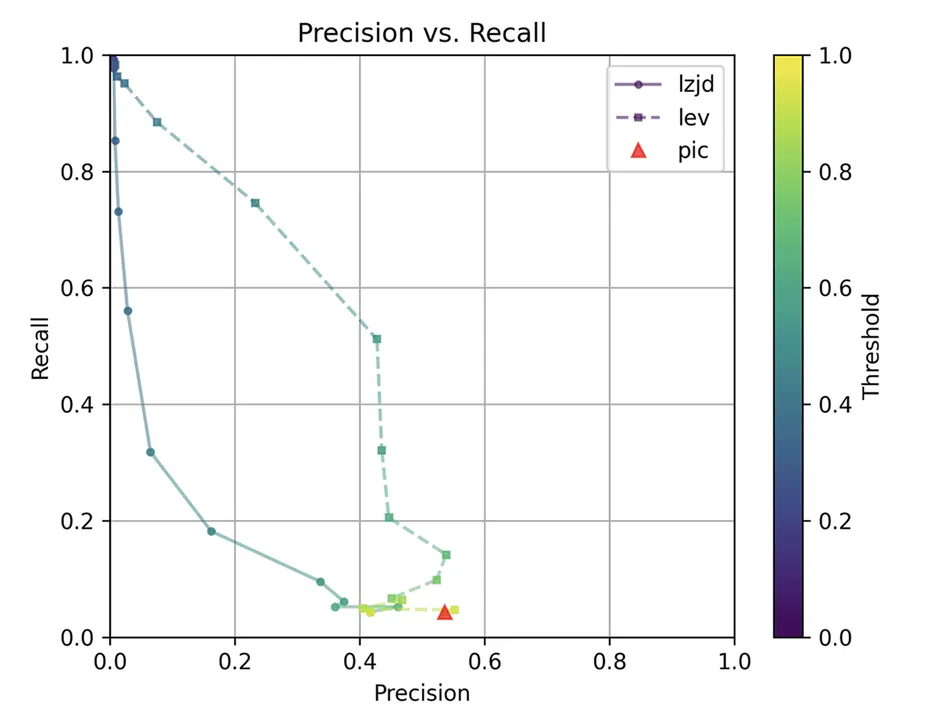
Determine 7: Precision vs. Recall Plot for “openssl -O1 vs -O2”
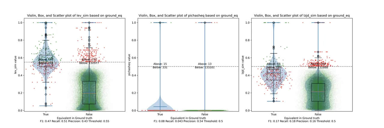
Determine 8: Violin Plot for “openssl -O1 vs -O2”. Click on to zoom in.
The precision vs. recall graph (Determine 7) is sort of attention-grabbing. PIC hashing begins at a precision of 0.54 and a recall of 0.043. LEV shoots straight up, indicating that by reducing the edge it’s potential to extend recall considerably with out dropping a lot precision. A very engaging tradeoff could be a precision of 0.43 and a recall of 0.51. That is the kind of tradeoff I hoped to see with fuzzy hashing.
Sadly, LZJD’s tradeoff line is once more not practically as interesting, because it curves within the flawed course.
We’ll say it is a fairly clear win for LEV.
Evaluating Optimization Ranges -O1 and -O3
Lastly, let’s examine -O1 and -O3, that are totally different, however each have the -fomit-frame-pointer possibility enabled by default.
Determine 9: Precision vs. Recall Plot for “openssl -O1 vs -O3”
Determine 10: Violin Plot for “openssl -O1 vs -O3”. Click on to zoom in.
These graphs look nearly similar to evaluating -O1 and -O2. I might describe the distinction between -O2 and -O3 as minor. So, it is once more a win for LEV.
Experiment 2: Totally different openssl Variations
The ultimate experiment I did was to check varied variations of openssl. Cory prompt this experiment as a result of he thought it was reflective of typical malware reverse engineering situations. The thought is that the malware creator launched Malware 1.0, which you reverse engineer. Later, the malware modifications a number of issues and releases Malware 1.1, and also you wish to detect which capabilities didn’t change so to keep away from reverse engineering them once more.
I in contrast a number of totally different variations of openssl:

I compiled every model utilizing gcc -g -O2.
openssl 1.0 and 1.1 are totally different minor variations of openssl. As defined right here:
Letter releases, corresponding to 1.0.2a, completely comprise bug and safety fixes and no new options.
So, we might count on that openssl 1.0.2u is pretty totally different from any 1.1.1 model. And, we might count on that in the identical minor model, 1.1.1 can be just like 1.1.1q, however it could be extra totally different than 1.1.1w.
Experiment 2a: openssl 1.0.2u vs 1.1.1w
As earlier than, let’s begin with essentially the most excessive comparability: 1.0.2u vs 1.1.1w.
Determine 11: Precision vs. Recall Plot for “openssl 1.0.2u vs 1.1.1w”
Determine 12: Violin Plot for “openssl 1.0.2u vs 1.1.1w”. Click on to zoom in.
Maybe not surprisingly, as a result of the 2 binaries are fairly totally different, all three methods wrestle. We’ll say it is a three means tie.
Experiment 2b: openssl 1.1.1 vs 1.1.1w
Now, let’s take a look at the unique 1.1.1 launch from September 2018 and examine it to the 1.1.1w bugfix launch from September 2023. Though plenty of time has handed between the releases, the one variations ought to be bug and safety fixes.
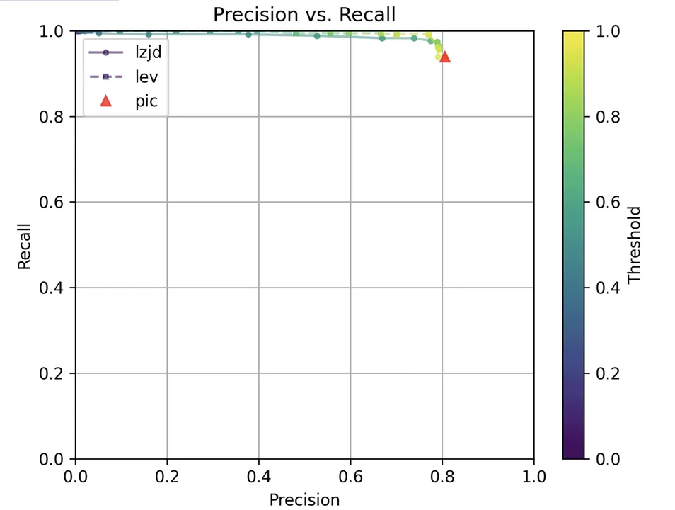
Determine 13: Precision vs. Recall Plot for “openssl 1.1.1 vs 1.1.1w”
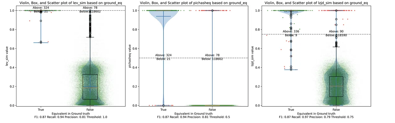
Determine 14: Violin Plot for “openssl 1.1.1 vs 1.1.1w”. Click on to zoom in.
All three methods do significantly better on this experiment, presumably as a result of there are far fewer modifications. PIC hashing achieves a precision of 0.75 and a recall of 0.71. LEV and LZJD go nearly straight up, indicating an enchancment in recall with minimal tradeoff in precision. At roughly the identical precision (0.75), LZJD achieves a recall of 0.82 and LEV improves it to 0.89. LEV is the clear winner, with LZJD additionally exhibiting a transparent benefit over PIC.
Experiment 2c: openssl 1.1.1q vs 1.1.1w
Let’s proceed taking a look at extra related releases. Now we’ll examine 1.1.1q from July 2022 to 1.1.1w from September 2023.
Determine 15: Precision vs. Recall Plot for “openssl 1.1.1q vs 1.1.1w”
Determine 16: Violin Plot for “openssl 1.1.1q vs 1.1.1w”. Click on to zoom in.
As may be seen within the precision vs. recall graph (Determine 15), PIC hashing begins at a powerful precision of 0.81 and a recall of 0.94. There merely is not plenty of room for LZJD or LEV to make an enchancment. This ends in a three-way tie.
Experiment second: openssl 1.1.1v vs 1.1.1w
Lastly, we’ll take a look at 1.1.1v and 1.1.1w, which have been launched solely a month aside.
Determine 17: Precision vs. Recall Plot for “openssl 1.1.1v vs 1.1.1w”
Determine 18: Violin Plot for “openssl 1.1.1v vs 1.1.1w”. Click on to zoom in.
Unsurprisingly, PIC hashing does even higher right here, with a precision of 0.82 and a recall of 1.0 (after rounding). Once more, there’s mainly no room for LZJD or LEV to enhance. That is one other three means tie.
Conclusions: Thresholds in Follow
We noticed some situations wherein LEV and LZJD outperformed PIC hashing. Nonetheless, it is vital to appreciate that we’re conducting these experiments with floor reality, and we’re utilizing the bottom reality to pick out the optimum threshold. You may see these thresholds listed on the backside of every violin plot. Sadly, should you look fastidiously, you will additionally discover that the optimum thresholds aren’t at all times the identical. For instance, the optimum threshold for LZJD within the “openssl 1.0.2u vs 1.1.1w” experiment was 0.95, but it surely was 0.75 within the “openssl 1.1.1q vs 1.1.1w” experiment.
In the actual world, to make use of LZJD or LEV, you should choose a threshold. In contrast to in these experiments, you might not choose the optimum one, since you would don’t have any means of figuring out in case your threshold was working properly or not. In the event you select a poor threshold, you may get considerably worse outcomes than PIC hashing.
PIC Hashing is Fairly Good
I believe we discovered that PIC hashing is fairly good. It isn’t excellent, but it surely typically offers wonderful precision. In idea, LZJD and LEV can carry out higher by way of recall, which is interesting. In apply, nevertheless, it could not be clear that they’d as a result of you wouldn’t know which threshold to make use of. Additionally, though we did not discuss a lot about computational efficiency, PIC hashing could be very quick. Though LZJD is a lot quicker than LEV, it is nonetheless not practically as quick as PIC.
Think about you’ve a database of one million malware perform samples and you’ve got a perform that you just wish to lookup within the database. For PIC hashing, that is simply an ordinary database lookup, which might profit from indexing and different precomputation methods. For fuzzy hash approaches, we would wish to invoke the similarity perform one million occasions every time we wished to do a database lookup.
There is a Restrict to Syntactic Similarity
Keep in mind that we included LEV to symbolize the optimum similarity based mostly on the edit distance of instruction bytes. LEV didn’t considerably outperform PIC , which is sort of telling, and suggests that there’s a elementary restrict to how properly syntactic similarity based mostly on instruction bytes can carry out. Surprisingly, PIC hashing seems to be near that restrict. We noticed a placing instance of this restrict when the body pointer was unintentionally omitted and, extra typically, all syntactic methods wrestle when the variations turn out to be too nice.
It’s unclear whether or not any variants, like computing similarities over meeting code as a substitute of executable code bytes, would carry out any higher.
The place Do We Go From Right here?
There are in fact different methods for evaluating similarity, corresponding to incorporating semantic info. Many researchers have studied this. The overall draw back to semantic methods is that they’re considerably costlier than syntactic methods. However, should you’re keen to pay the upper computational value, you may get higher outcomes.
Lately, a significant new characteristic known as BSim was added to Ghidra. BSim can discover structurally related capabilities in probably massive collections of binaries or object recordsdata. BSim relies on Ghidra’s decompiler and may discover matches throughout compilers used, architectures, and/or small modifications to supply code.
One other attention-grabbing query is whether or not we are able to use neural studying to assist compute similarity. For instance, we would be capable to prepare a mannequin to know that omitting the body pointer doesn’t change the which means of a perform, and so should not be counted as a distinction.