
Think about that you just reverse engineered a bit of malware in painstaking element solely to seek out that the malware writer created a barely modified model of the malware the following day. You would not wish to redo all of your arduous work. One strategy to keep away from beginning over from scratch is to make use of code comparability strategies to attempt to establish pairs of features within the previous and new model which are “the identical.” (I’ve used quotes as a result of “identical” on this occasion is a little bit of a nebulous idea, as we’ll see).
A number of instruments may also help in such conditions. A very talked-about industrial software is zynamics’ BinDiff, which is now owned by Google and is free. The SEI’s Pharos binary evaluation framework additionally features a code comparability utility known as fn2hash. On this SEI Weblog publish, the primary in a two-part collection on hashing, I first clarify the challenges of code comparability and current our answer to the issue. I then introduce fuzzy hashing, a brand new kind of hashing algorithm that may carry out inexact matching. Lastly, I examine the efficiency of fn2hash and a fuzzy hashing algorithm utilizing a variety of experiments.
Background
Actual Hashing
fn2hash employs a number of forms of hashing. Essentially the most generally used known as place impartial code (PIC) hashing. To see why PIC hashing is necessary, we’ll begin by a naive precursor to PIC hashing: merely hashing the instruction bytes of a perform. We’ll name this precise hashing.
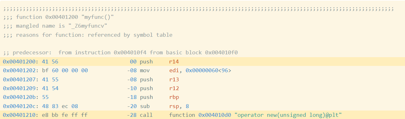
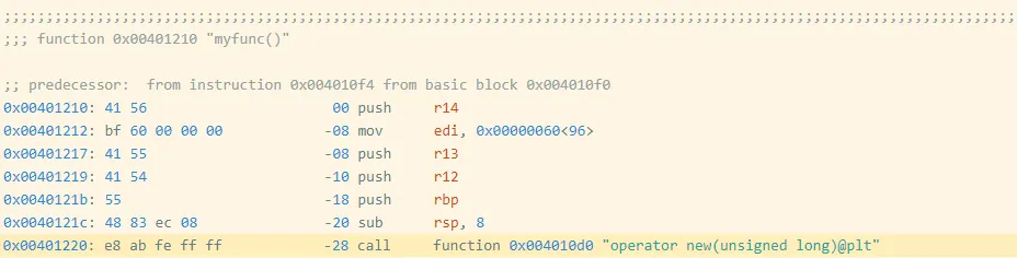
For example, I compiled this straightforward program oo.cpp with g++. Determine 1 reveals the start of the meeting code for the perform myfunc (full code):
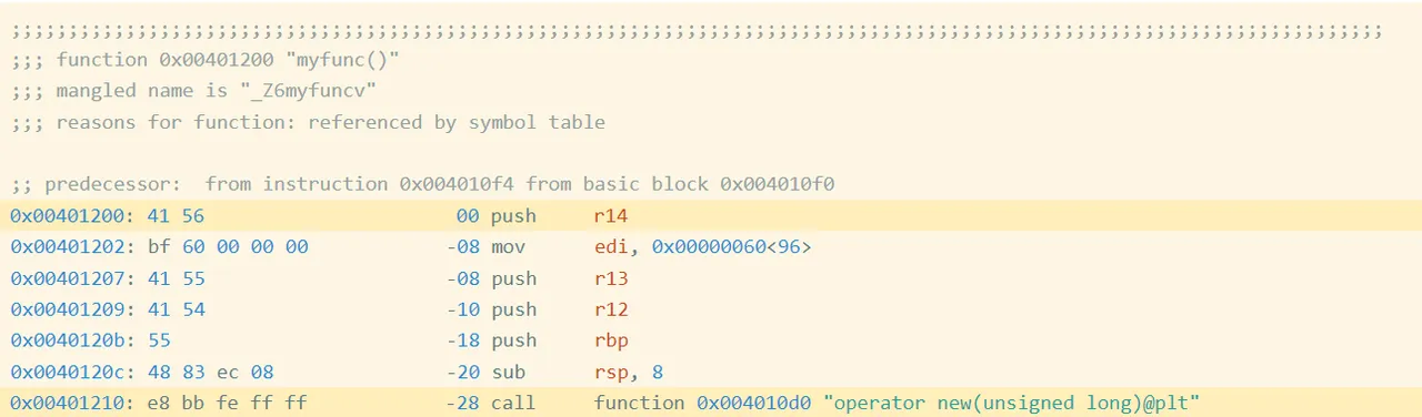
Determine 1: Meeting Code and Bytes from oo.gcc
Actual Bytes
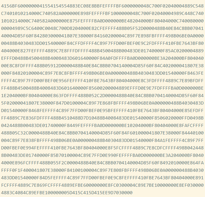
Within the first highlighted line of Determine 1, you’ll be able to see that the primary instruction is a push r14, which is encoded by the hexadecimal instruction bytes 41 56. If we accumulate the encoded instruction bytes for each instruction within the perform, we get the next (Determine 2):
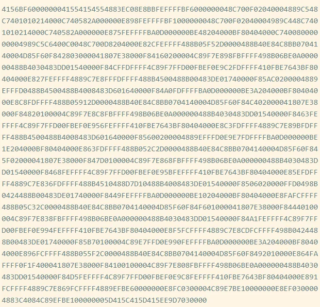
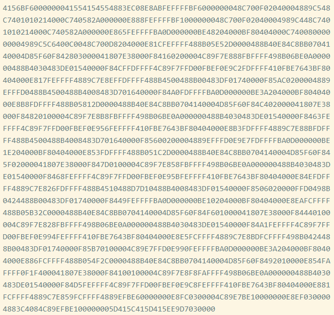
Determine 2: Actual Bytes in oo.gcc
We name this sequence the precise bytes of the perform. We will hash these bytes to get an precise hash, 62CE2E852A685A8971AF291244A1283A.
Shortcomings of Actual Hashing
The highlighted name at deal with 0x401210 is a relative name, which signifies that the goal is specified as an offset from the present instruction (technically, the following instruction). When you take a look at the instruction bytes for this instruction, it contains the bytes bb fe ff ff, which is 0xfffffebb in little endian kind. Interpreted as a signed integer worth, that is -325. If we take the deal with of the following instruction (0x401210 + 5 == 0x401215) after which add -325 to it, we get 0x4010d0, which is the deal with of operator new, the goal of the decision. Now we all know that bb fe ff ff is an offset from the following instruction. Such offsets are known as relative offsets as a result of they’re relative to the deal with of the following instruction.
I created a barely modified program (oo2.gcc) by including an empty, unused perform earlier than myfunc (Determine 3). You could find the disassembly of myfunc for this executable right here.
If we take the precise hash of myfunc on this new executable, we get 05718F65D9AA5176682C6C2D5404CA8D. You’ll discover that is completely different from the hash for myfunc within the first executable, 62CE2E852A685A8971AF291244A1283A. What occurred? Let’s take a look at the disassembly.
Determine 3: Meeting Code and Bytes from oo2.gcc
Discover that myfunc moved from 0x401200 to 0x401210, which additionally moved the deal with of the decision instruction from 0x401210 to 0x401220. The decision goal is specified as an offset from the (subsequent) instruction’s deal with, which modified by 0x10 == 16, so the offset bytes for the decision modified from bb fe ff ff (-325) to ab fe ff ff (-341 == -325 – 16). These adjustments modify the precise bytes as proven in Determine 4.
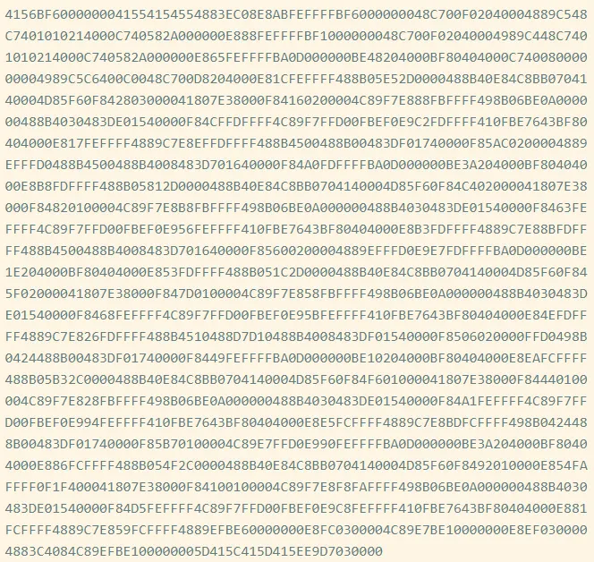
Determine 4: Actual Bytes in oo2.gcc
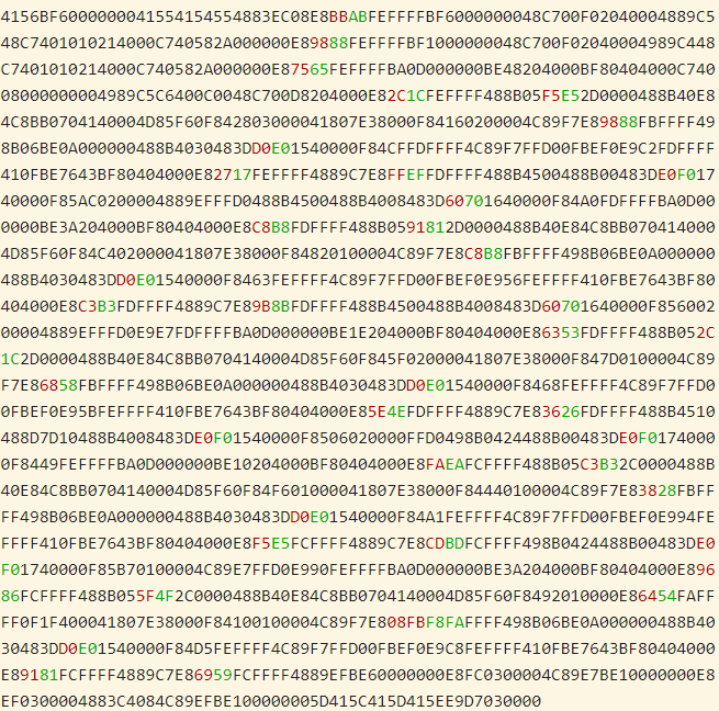
Determine 5 presents a visible comparability. Purple represents bytes which are solely in oo.gcc, and inexperienced represents bytes in oo2.gcc. The variations are small as a result of the offset is simply altering by 0x10, however this is sufficient to break precise hashing.
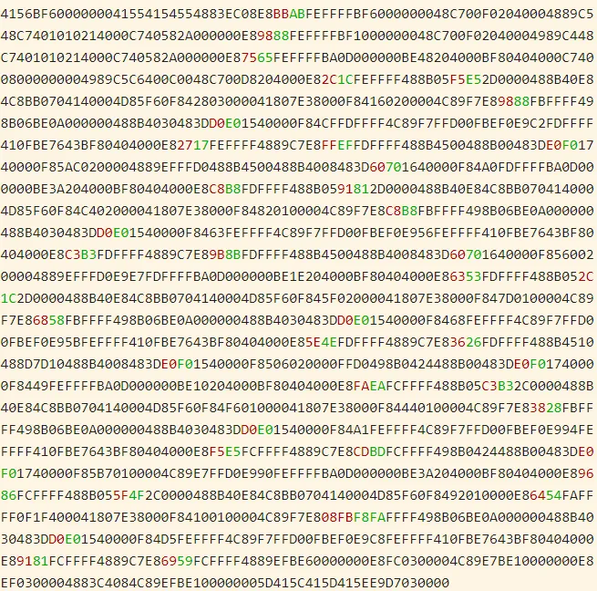
Determine 5: Distinction Between Actual Bytes in oo.gcc and oo2.gcc
PIC Hashing
The objective of PIC hashing is to compute a hash or signature of code in a manner that preserves the hash when relocating the code. This requirement is necessary as a result of, as we simply noticed, modifying a program usually ends in small adjustments to addresses and offsets, and we do not need these adjustments to switch the hash. The instinct behind PIC hashing is very straight-forward: Establish offsets and addresses which are more likely to change if this system is recompiled, resembling bb fe ff ff, and easily set them to zero earlier than hashing the bytes. That manner, if they modify as a result of the perform is relocated, the perform’s PIC hash will not change.
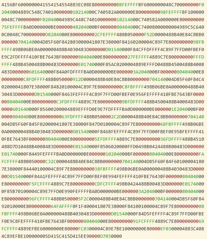
The next visible diff (Determine 6) reveals the variations between the precise bytes and the PIC bytes on myfunc in oo.gcc. Purple represents bytes which are solely within the PIC bytes, and inexperienced represents the precise bytes. As anticipated, the primary change we are able to see is the byte sequence bb fe ff ff, which is modified to zeros.

Determine 6: Byte Distinction Between PIC Bytes (Purple) and Actual Bytes (Inexperienced)
If we hash the PIC bytes, we get the PIC hash EA4256ECB85EDCF3F1515EACFA734E17. And, as we’d hope, we get the identical PIC hash for myfunc within the barely modified oo2.gcc.
Evaluating the Accuracy of PIC Hashing
The first motivation behind PIC hashing is to detect an identical code that’s moved to a distinct location. However what if two items of code are compiled with completely different compilers or completely different compiler flags? What if two features are very related, however one has a line of code eliminated? These adjustments would modify the non-offset bytes which are used within the PIC hash, so it might change the PIC hash of the code. Since we all know that PIC hashing is not going to all the time work, on this part we talk about the right way to measure the efficiency of PIC hashing and examine it to different code comparability strategies.
Earlier than we are able to outline the accuracy of any code comparability approach, we’d like some floor fact that tells us which features are equal. For this weblog publish, we use compiler debug symbols to map perform addresses to their names. Doing so offers us with a floor fact set of features and their names. Additionally, for the needs of this weblog publish, we assume that if two features have the identical identify, they’re “the identical.” (This, clearly, shouldn’t be true normally!)
Confusion Matrices
So, to illustrate we’ve two related executables, and we wish to consider how properly PIC hashing can establish equal features throughout each executables. We begin by contemplating all potential pairs of features, the place every pair incorporates a perform from every executable. This method known as the Cartesian product between the features within the first executable and the features within the second executable. For every perform pair, we use the bottom fact to find out whether or not the features are the identical by seeing if they’ve the identical identify. We then use PIC hashing to foretell whether or not the features are the identical by computing their hashes and seeing if they’re an identical. There are two outcomes for every dedication, so there are 4 prospects in complete:
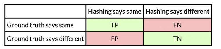
- True constructive (TP): PIC hashing accurately predicted the features are equal.
- True destructive (TN): PIC hashing accurately predicted the features are completely different.
- False constructive (FP): PIC hashing incorrectly predicted the features are equal, however they don’t seem to be.
- False destructive (FN): PIC hashing incorrectly predicted the features are completely different, however they’re equal.
To make it just a little simpler to interpret, we colour the nice outcomes inexperienced and the dangerous outcomes purple. We will signify these in what known as a confusion matrix:

For instance, here’s a confusion matrix from an experiment by which I take advantage of PIC hashing to check openssl variations 1.1.1w and 1.1.1v when they’re each compiled in the identical manner. These two variations of openssl are fairly related, so we’d count on that PIC hashing would do properly as a result of quite a lot of features can be an identical however shifted to completely different addresses. And, certainly, it does:

Metrics: Accuracy, Precision, and Recall
So, when does PIC hashing work properly and when does it not? To reply these questions, we will want a neater strategy to consider the standard of a confusion matrix as a single quantity. At first look, accuracy looks as if probably the most pure metric, which tells us: What number of pairs did hashing predict accurately? This is the same as
For the above instance, PIC hashing achieved an accuracy of
You may assume 99.9 p.c is fairly good, however for those who look intently, there’s a refined downside: Most perform pairs are not equal. In accordance with the bottom fact, there are TP + FN = 344 + 1 = 345 equal perform pairs, and TN + FP = 118,602 + 78 = 118,680 nonequivalent perform pairs. So, if we simply guessed that each one perform pairs have been nonequivalent, we’d nonetheless be proper 118680 / (118680 + 345) = 99.9 p.c of the time. Since accuracy weights all perform pairs equally, it isn’t probably the most applicable metric.
As an alternative, we wish a metric that emphasizes constructive outcomes, which on this case are equal perform pairs. This result’s in line with our objective in reverse engineering, as a result of understanding that two features are equal permits a reverse engineer to switch data from one executable to a different and save time.
Three metrics that focus extra on constructive circumstances (i.e., equal features) are precision, recall, and F1 rating:
- Precision: Of the perform pairs hashing declared equal, what number of have been really equal? This is the same as TP / (TP + FP).
- Recall: Of the equal perform pairs, what number of did hashing accurately declare as equal? This is the same as TP / (TP + FN).
- F1 rating: This can be a single metric that displays each the precision and recall. Particularly, it’s the harmonic imply of the precision and recall, or (2 ∗ Recall ∗ Precision) / (Recall + Precision). In comparison with the arithmetic imply, the harmonic imply is extra delicate to low values. Which means that if both the precision or recall is low, the F1 rating may even be low.
So, wanting on the instance above, we are able to compute the precision, recall, and F1 rating. The precision is 344 / (344 + 78) = 0.81, the recall is 344 / (344 + 1) = 0.997, and the F1 rating is 2 ∗ 0.81 ∗ 0.997 / (0.81 + 0.997) = 0.89. PIC hashing is ready to establish 81 p.c of equal perform pairs, and when it does declare a pair is equal it’s appropriate 99.7 p.c of the time. This corresponds to an F1 rating of 0.89 out of 1.0, which is fairly good.
Now, you may be questioning how properly PIC hashing performs when there are extra substantial variations between executables. Let’s take a look at one other experiment. On this one, I examine an openssl executable compiled with GCC to at least one compiled with Clang. As a result of GCC and Clang generate meeting code in another way, we’d count on there to be much more variations.
Here’s a confusion matrix from this experiment:
On this instance, PIC hashing achieved a recall of 23 / (23 + 301) = 0.07, and a precision of 23 / (23 + 31) = 0.43. So, PIC hashing can solely establish 7 p.c of equal perform pairs, however when it does declare a pair is equal it’s appropriate 43 p.c of the time. This corresponds to an F1 rating of 0.12 out of 1.0, which is fairly dangerous. Think about that you just spent hours reverse engineering the 324 features in one of many executables solely to seek out that PIC hashing was solely in a position to establish 23 of them within the different executable. So, you’ll be pressured to needlessly reverse engineer the opposite features from scratch. Can we do higher?
The Nice Fuzzy Hashing Debate
Within the subsequent publish on this collection, we are going to introduce a really completely different kind of hashing known as fuzzy hashing, and discover whether or not it might probably yield higher efficiency than PIC hashing alone. As with PIC hashing, fuzzy hashing reads a sequence of bytes and produces a hash. In contrast to PIC hashing, nonetheless, once you examine two fuzzy hashes, you’re given a similarity worth between 0.0 and 1.0, the place 0.0 means utterly dissimilar, and 1.0 means utterly related. We are going to current the outcomes of a number of experiments that pit PIC hashing and a preferred fuzzy hashing algorithm in opposition to one another and study their strengths and weaknesses within the context of malware reverse-engineering.